1 Goals for Lab 02

Review dplyr functions learned in last lab and DataCamp course
Practice using dplyr functions to get to know a new dataset
Map global plot aesthetics to variables in ggplot2
Create facetted plots with ggplot2

2 Slides for today

knitr::include_url("slides/02-slides.html")

3 Inspiration + data

We’ll use data from the Museum of Modern Art (MoMA)

Publicly available on GitHub
As analyzed by fivethirtyeight.com
And by others

4 Packages needed

library(here) # to set file path if working from local file
library(tidyverse) # readr, ggplot2, dplyr

5 Read in the data

Note! This is not the original data- I did a lot of cleaning and decision-making in the pre-processing. The below contains only paintings and drawings in the MoMA collection.

Use this code chunk to read in the data available at http://bit.ly/cs631-moma:

library(readr)
moma <- read_csv("http://bit.ly/cs631-moma")

I called my cleaned data artworks-cleaned.csv, and stored it in a folder called data. You can use this code if you want to read in the local CSV file.

library(here)
library(readr)
library(dplyr)
moma <- read_csv(here::here("data", "artworks-cleaned.csv"))

6 Know your data

Challenge #1:

Try to answer all of these questions using dplyr. Answers are below but try them on your own first!

How many paintings (rows) are in moma? How many variables (columns) are in moma?
What is the first painting acquired by MoMA? Which year? Which artist? What title?
What is the oldest painting in the collection? Which year? Which artist? What title?
How many distinct artists are there?
Which artist has the most paintings in the collection? How many paintings are by this artist?
How many paintings by male vs female artists?

If you want more:

How many artists of each gender are there?
In what year were the most paintings acquired? Created?
In what year was the first painting by a (solo) female artist acquired? When was that painting created? Which artist? What title?

6.1 How many paintings?

How many rows/observations are in moma?
How many variables are in moma?

Hint: These questions can be answered using the dplyr function glimpse.

library(dplyr)
moma

# A tibble: 2,253 x 23
   title  artist  artist_bio artist_birth_ye… artist_death_ye… num_artists
   <chr>  <chr>   <chr>                 <dbl>            <dbl>       <dbl>
 1 Rope … Joan M… (Spanish,…            1893.            1983.          1.
 2 Fire … Paul K… (German, …            1879.            1940.          1.
 3 Portr… Paul K… (German, …            1879.            1940.          1.
 4 Guitar Pablo … (Spanish,…            1881.            1973.          1.
 5 Grand… Arthur… (American…            1880.            1946.          1.
 6 "\"M'… Franci… (French, …            1879.            1953.          1.
 7 Untit… Blinky… (German, …            1943.            1977.          1.
 8 Dayli… Pierre… (French, …            1880.            1950.          1.
 9 The B… Paul C… (French, …            1839.            1906.          1.
10 Synth… Enrico… (Italian,…            1894.            1956.          1.
# ... with 2,243 more rows, and 17 more variables: n_female_artists <dbl>,
#   n_male_artists <dbl>, artist_gender <chr>, year_acquired <dbl>,
#   year_created <dbl>, circumference_cm <lgl>, depth_cm <dbl>,
#   diameter_cm <lgl>, height_cm <dbl>, length_cm <lgl>, width_cm <dbl>,
#   seat_height_cm <lgl>, purchase <lgl>, gift <lgl>, exchange <lgl>,
#   classification <chr>, department <chr>

glimpse(moma)

Observations: 2,253
Variables: 23
$ title             <chr> "Rope and People, I", "Fire in the Evening",...
$ artist            <chr> "Joan Miró", "Paul Klee", "Paul Klee", "Pabl...
$ artist_bio        <chr> "(Spanish, 1893–1983)", "(German, born Switz...
$ artist_birth_year <dbl> 1893, 1879, 1879, 1881, 1880, 1879, 1943, 18...
$ artist_death_year <dbl> 1983, 1940, 1940, 1973, 1946, 1953, 1977, 19...
$ num_artists       <dbl> 1, 1, 1, 1, 1, 1, 1, 1, 1, 1, 1, 1, 1, 1, 1,...
$ n_female_artists  <dbl> 0, 0, 0, 0, 0, 0, 0, 0, 0, 0, 0, 0, 0, 0, 0,...
$ n_male_artists    <dbl> 1, 1, 1, 1, 1, 1, 1, 1, 1, 1, 1, 1, 1, 1, 1,...
$ artist_gender     <chr> "Male", "Male", "Male", "Male", "Male", "Mal...
$ year_acquired     <dbl> 1936, 1970, 1966, 1955, 1939, 1968, 1997, 19...
$ year_created      <dbl> 1935, 1929, 1927, 1919, 1925, 1919, 1970, 19...
$ circumference_cm  <lgl> NA, NA, NA, NA, NA, NA, NA, NA, NA, NA, NA, ...
$ depth_cm          <dbl> NA, NA, NA, NA, NA, NA, NA, NA, NA, NA, NA, ...
$ diameter_cm       <lgl> NA, NA, NA, NA, NA, NA, NA, NA, NA, NA, NA, ...
$ height_cm         <dbl> 104.8, 33.8, 60.3, 215.9, 50.8, 129.2, 200.0...
$ length_cm         <lgl> NA, NA, NA, NA, NA, NA, NA, NA, NA, NA, NA, ...
$ width_cm          <dbl> 74.6, 33.3, 36.8, 78.7, 54.0, 89.9, 200.0, 3...
$ seat_height_cm    <lgl> NA, NA, NA, NA, NA, NA, NA, NA, NA, NA, NA, ...
$ purchase          <lgl> FALSE, FALSE, FALSE, FALSE, FALSE, FALSE, FA...
$ gift              <lgl> TRUE, FALSE, FALSE, TRUE, TRUE, FALSE, TRUE,...
$ exchange          <lgl> FALSE, FALSE, FALSE, FALSE, TRUE, FALSE, FAL...
$ classification    <chr> "Painting", "Painting", "Painting", "Paintin...
$ department        <chr> "Painting & Sculpture", "Painting & Sculptur...

There are 2253 paintings in moma.

6.2 What is the first painting acquired?

What is the first painting acquired by MoMA (since they started tracking)?
What year was it acquired?
Which artist?
What title?

Hint: These questions can be answered by combining two dplyr functions: select and arrange.

moma %>% 
  select(artist, title, year_acquired) %>% 
  arrange(year_acquired)

# A tibble: 2,253 x 3
   artist            title                                   year_acquired
   <chr>             <chr>                                           <dbl>
 1 Edward Hopper     House by the Railroad                           1930.
 2 Bernard Karfiol   Seated Nude                                     1930.
 3 Pierre Roy        Daylight Savings Time                           1931.
 4 Preston Dickinson Plums on a Plate                                1931.
 5 Otto Dix          Dr. Mayer-Hermann                               1932.
 6 Paul Cézanne      The Bather                                      1934.
 7 Paul Cézanne      Pines and Rocks (Fontainebleau?)                1934.
 8 Paul Cézanne      Still Life with Ginger Jar, Sugar Bowl…         1934.
 9 Paul Cézanne      Still Life with Apples                          1934.
10 Arthur B. Davies  Italian Landscape                               1934.
# ... with 2,243 more rows

6.3 What is the oldest painting in the MoMA collection?

What is the oldest painting in the MoMA collection historically (since they started tracking)?
What year was it created?
Which artist?
What title?

Hint: These questions can be answered by combining two dplyr functions: select and arrange.

moma %>% 
  select(artist, title, year_created) %>% 
  arrange(year_created)

# A tibble: 2,253 x 3
   artist       title                                    year_created
   <chr>        <chr>                                           <dbl>
 1 Odilon Redon Landscape at Daybreak                           1872.
 2 Odilon Redon Apache (Man on Horseback)                       1875.
 3 Odilon Redon Apache (Man on Horseback II)                    1875.
 4 Odilon Redon Fishing Boat                                    1875.
 5 Odilon Redon Rocky Peak                                      1875.
 6 Odilon Redon The Rocky Slope                                 1875.
 7 Odilon Redon Landscape with Rocks, near Royan                1875.
 8 Paul Cézanne Still Life with Fruit Dish                      1879.
 9 Paul Cézanne L'Estaque                                       1879.
10 Claude Monet On the Cliff at Pourville, Clear Weather        1882.
# ... with 2,243 more rows

To do inline comments, I could say that the oldest painting is Landscape at Daybreak, painted by Odilon Redon in 1872.

6.4 How many artists?

How many distinct artists are there?

Hint: Try dplyr::distinct.

moma %>% 
  distinct(artist)

# A tibble: 989 x 1
   artist           
   <chr>            
 1 Joan Miró        
 2 Paul Klee        
 3 Pablo Picasso    
 4 Arthur Dove      
 5 Francis Picabia  
 6 Blinky Palermo   
 7 Pierre Roy       
 8 Paul Cézanne     
 9 Enrico Prampolini
10 Jankel Adler     
# ... with 979 more rows

You could add a tally() too to get just the number of rows. You can also then use pull() to get that single number out of the tibble:

num_artists <- moma %>% 
  distinct(artist) %>% 
  tally() %>% 
  pull()
num_artists

[1] 989

Then I can refer to this number in inline comments like: there are 989 total.

6.5 Which artist has the most paintings?

Which artist has the most paintings ever owned by moma?
How many paintings in the MoMA collection by that artist?

Hint: Try dplyr::count. Use ?count to figure out how to sort the output.

moma %>% 
  count(artist, sort = TRUE)

# A tibble: 989 x 2
   artist               n
   <chr>            <int>
 1 Pablo Picasso       55
 2 Henri Matisse       32
 3 On Kawara           32
 4 Jacob Lawrence      30
 5 Batiste Madalena    25
 6 Jean Dubuffet       25
 7 Odilon Redon        25
 8 Ben Vautier         24
 9 Frank Stella        23
10 Philip Guston       23
# ... with 979 more rows

In the ?count documentation, it says: “count and tally are designed so that you can call them repeatedly, each time rolling up a level of detail.” Try running count() again (leave parentheses empty) on your last code chunk.

moma %>% 
  count(artist, sort = TRUE) %>% 
  count()

# A tibble: 1 x 1
     nn
  <int>
1   989

6.6 How many paintings by male vs female artists?

moma %>% 
  count(artist_gender)

# A tibble: 3 x 2
  artist_gender     n
  <chr>         <int>
1 Female          252
2 Male           1991
3 <NA>             10

Now together we’ll count the number of artists by gender. You’ll need to give count two variable names in the parentheses: artist_gender and artist.

moma %>% 
  count(artist_gender, artist, sort = TRUE)

# A tibble: 989 x 3
   artist_gender artist               n
   <chr>         <chr>            <int>
 1 Male          Pablo Picasso       55
 2 Male          Henri Matisse       32
 3 Male          On Kawara           32
 4 Male          Jacob Lawrence      30
 5 Male          Batiste Madalena    25
 6 Male          Jean Dubuffet       25
 7 Male          Odilon Redon        25
 8 Male          Ben Vautier         24
 9 Male          Frank Stella        23
10 Male          Philip Guston       23
# ... with 979 more rows

This output is not superhelpful as we already know that Pablo Picasso has 55 paintings in the MoMA collection. But how can we find out which female artist has the most paintings? We have a few options. Let’s first add a filter for females.

moma %>% 
  count(artist_gender, artist, sort = TRUE) %>% 
  filter(artist_gender == "Female")

# A tibble: 143 x 3
   artist_gender artist                    n
   <chr>         <chr>                 <int>
 1 Female        Sherrie Levine           12
 2 Female        Agnes Martin              9
 3 Female        Elizabeth Murray          8
 4 Female        Susan Rothenberg          8
 5 Female        Joan Mitchell             6
 6 Female        Loren MacIver             6
 7 Female        R. H. Quaytman            6
 8 Female        Helen Frankenthaler       5
 9 Female        Georgia O'Keeffe          4
10 Female        Lynette Yiadom-Boakye     4
# ... with 133 more rows

Another option is to use another dplyr function called top_n(). Use ?top_n to see how it works. How it won’t work in this context:

moma %>% 
  count(artist_gender, artist, sort = TRUE) %>% 
  top_n(2)

# A tibble: 3 x 3
  artist_gender artist            n
  <chr>         <chr>         <int>
1 Male          Pablo Picasso    55
2 Male          Henri Matisse    32
3 Male          On Kawara        32

How it will work better is following a group_by(artist_gender):

moma %>% 
  count(artist_gender, artist, sort = TRUE) %>% 
  group_by(artist_gender) %>% 
  top_n(1)

# A tibble: 3 x 3
# Groups:   artist_gender [3]
  artist_gender artist                                                 n
  <chr>         <chr>                                              <int>
1 Male          Pablo Picasso                                         55
2 Female        Sherrie Levine                                        12
3 <NA>          Gilbert & George, Gilbert Proesch, George Passmore     2

Now we can see that Sherrie Levine has 12 paintings. This is a pretty far cry from the 55 paintings by Pablo Picasso.

6.7 How many artists of each gender are there?

This is a harder question to answer than you think! This is because the level of observation in our current moma dataset is unique paintings. We have multiple paintings done by the same artists though, so counting just the number of unique paintings is different than counting the number of unique artists.

Remember how count can be used back-to-back to roll up a level of detail? Try running count(artist_gender) again on your last code chunk.

moma %>% 
  count(artist_gender, artist) %>% 
  count(artist_gender)

# A tibble: 3 x 2
  artist_gender    nn
  <chr>         <int>
1 Female          143
2 Male            837
3 <NA>              9

This output takes the previous table (made with count(artist_gender, artist)), and essentially ignores the n column. So we no longer care about how many paintings each individual artist created. Instead, we want to count the rows in this new table where each row is a unique artist. By counting by artist_gender in the last line, we are grouping by levels of that variable (so Female/Male/NA) and nn is the number of unique artists for each gender category recorded.

6.8 When were the most paintings in the collection acquired?

Hint: Try dplyr::count. Use ?count to figure out how to sort the output.

moma %>% 
  count(year_acquired, sort = TRUE)

# A tibble: 88 x 2
   year_acquired     n
           <dbl> <int>
 1         1985.    86
 2         1942.    71
 3         1979.    71
 4         1991.    67
 5         2005.    67
 6         1967.    65
 7         2008.    55
 8         1961.    45
 9         1969.    45
10         1956.    42
# ... with 78 more rows

6.9 When were the most paintings in the collection created?

Hint: Try dplyr::count. Use ?count to figure out how to sort the output.

moma %>% 
  count(year_created, sort = TRUE)

# A tibble: 139 x 2
   year_created     n
          <dbl> <int>
 1        1977.    57
 2        1940.    56
 3        1964.    56
 4        1961.    50
 5        1962.    49
 6        1963.    44
 7        1959.    42
 8        1968.    40
 9        1960.    39
10        1914.    37
# ... with 129 more rows

6.10 What about the first painting by a solo female artist?

Hint: Try combining three dplyr functions: filter, select, and arrange.

When was the first painting by a solo female artist acquired?

moma %>% 
  filter(num_artists == 1 & n_female_artists == 1) %>% 
  select(title, artist, year_acquired, year_created) %>% 
  arrange(year_acquired)

# A tibble: 252 x 4
   title                           artist       year_acquired year_created
   <chr>                           <chr>                <dbl>        <dbl>
 1 Landscape, 47                   Natalia Gon…         1937.        1912.
 2 Shack                           Loren MacIv…         1938.        1934.
 3 Hopscotch                       Loren MacIv…         1940.        1940.
 4 Shadows with Painting           Irene Rice …         1941.        1940.
 5 Figure                          Varvara Ste…         1941.        1921.
 6 Still Life in Red               Amelia Pelá…         1942.        1938.
 7 White Lines                     Irene Rice …         1942.        1942.
 8 Musical Squash                  Maud Morgan          1942.        1942.
 9 Desolation                      Raquel Forn…         1942.        1942.
10 Self-Portrait with Cropped Hair Frida Kahlo          1943.        1940.
# ... with 242 more rows

What is the oldest painting by a solo female artist, and when was it created?

moma %>% 
  filter(num_artists == 1 & n_female_artists == 1) %>% 
  select(title, artist, year_acquired, year_created) %>% 
  arrange(year_created)

# A tibble: 252 x 4
   title                          artist        year_acquired year_created
   <chr>                          <chr>                 <dbl>        <dbl>
 1 Self-Portrait with Two Flower… Paula Moders…         2017.        1907.
 2 Girl with Bare Shoulders       Gwen John             1958.        1909.
 3 Girl Reading at a Window       Gwen John             1971.        1911.
 4 Landscape, 47                  Natalia Gonc…         1937.        1912.
 5 Cubist Nude                    Alexandra Ex…         1991.        1912.
 6 Rayonism, Blue-Green Forest    Natalia Gonc…         1985.        1913.
 7 The Factory and the Bridge     Olga Rozanova         1985.        1913.
 8 Subject from a Dyer's Shop     Lyubov Popova         1985.        1914.
 9 Portuguese Market              Sonia Delaun…         1955.        1915.
10 Girl with a Blue Scarf         Gwen John             1963.        1915.
# ... with 242 more rows

# or, because artist_gender is missing when num_artists > 1
moma %>% 
  filter(artist_gender == "Female") %>% 
  select(title, artist, year_acquired, year_created) %>% 
  arrange(year_acquired)

7 Basics of `ggplot2`

Challenge #2:

We’ll do this together (nothing to turn in): see slides.

8 Plot your data

8.1 Plot year painted vs year acquired

Challenge #3:

Let’s recreate this plot from fivethirtyeight (mostly)!

Things to consider:

You’ll want to play around with setting an alpha value here- keep in mind that 0 is totally transparent and 1 is opaque.
Try using geom_abline() to add the line in red (use the default intercept value of 0). The actual red line is difficult to recreate- here is what the authors say: “The red regression line shows the “modernizing” of MoMA’s collection — how quickly the museum has moved toward acquiring recent paintings.”
Go back to Lab 01 to review how to do the following:
- Change the x- and y-axis labels and the plot title to match the plot above

ggplot(moma, aes(year_created, year_acquired)) +
  geom_point(alpha = .1, na.rm = TRUE) +
  geom_abline(intercept = c(0,0), colour = "red") +
  labs(x = "Year Painted", y = "Year Acquired") +
  ggtitle("MoMA Keeps Its Collection Current")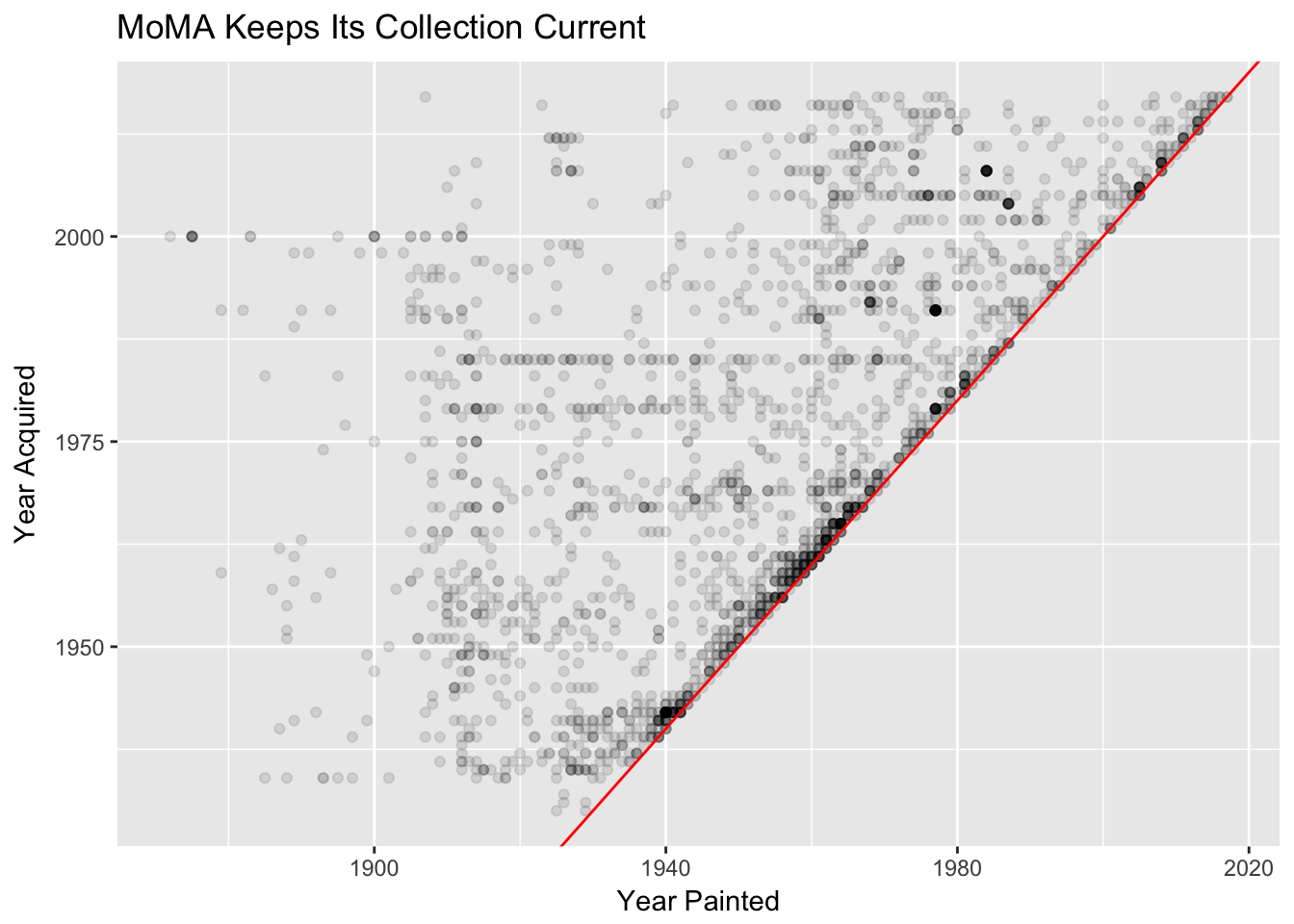

8.2 Facet by artist gender

Can you make the same plot above, but facet by artist gender?

Hint: For this to make sense, you probably want to do some filtering to select only those paintings where there was one “solo” artist.

moma_solo <- moma %>% 
  filter(num_artists == 1)
ggplot(moma_solo, aes(year_created, year_acquired)) +
  geom_point(alpha = .1) +
  geom_abline(intercept = c(0,0), colour = "red") +
  labs(x = "Year Painted", y = "Year Acquired") +
  ggtitle("MoMA Keeps Its Collection Current") +
  facet_wrap(~artist_gender)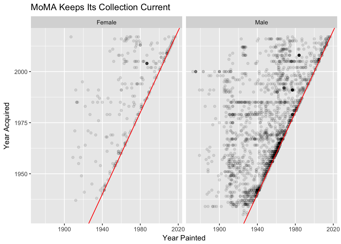

9 Plot painting dimensions

Challenge #4:

Let’s (somewhat) try to recreate this scatterplot from fivethirtyeight.

To recreate, some things to consider:

Try filtering all paintings with height less than 600 cm and width less than 760 cm.
If you want to add color as in the original, you’ll need to create a new variable using mutate.

Hint: You’ll probably also want to look into case_when to create a categorical variable to color by.

moma_dim <- moma %>% 
  filter(height_cm < 600, width_cm < 760) %>% 
  mutate(hw_ratio = height_cm / width_cm,
         hw_cat = case_when(
           hw_ratio > 1 ~ "taller than wide",
           hw_ratio < 1 ~ "wider than tall",
           hw_ratio == 1 ~ "perfect square"
         ))
library(ggthemes)
ggplot(moma_dim, aes(x = width_cm, y = height_cm, colour = hw_cat)) +
  geom_point(alpha = .5) +
  ggtitle("MoMA Paintings, Tall and Wide") +
  scale_colour_manual(name = "",
                      values = c("gray50", "#FF9900", "#B14CF0")) +
  theme_fivethirtyeight() +
  theme(axis.title = element_text()) +
  labs(x = "Width", y = "Height")

Because Grace is right, we can do better with colors!

library(ggthemes)
ggplot(moma_dim, aes(x = width_cm, y = height_cm, colour = hw_cat)) +
  geom_point(alpha = .5) +
  ggtitle("MoMA Paintings, Tall and Wide") +
  scale_colour_manual(name = "",
                      values = c("gray50", "#ee5863", "#6999cd")) +
  theme_fivethirtyeight() +
  theme(axis.title = element_text()) +
  labs(x = "Width", y = "Height")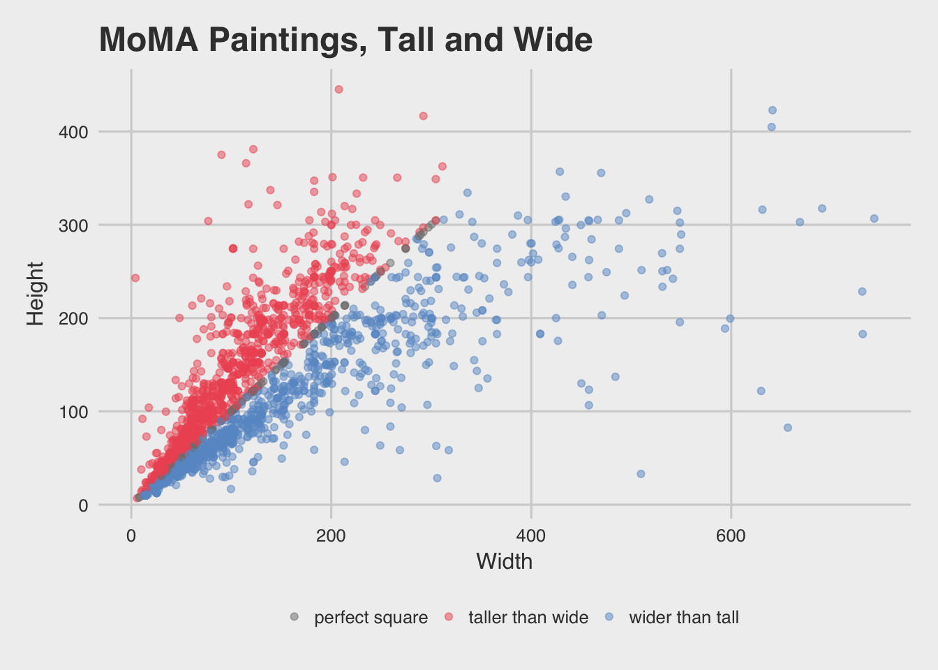

We could also do away with the legend and use geom_annotate instead.

library(ggthemes)
ggplot(moma_dim, aes(x = width_cm, y = height_cm, colour = hw_cat)) +
  geom_point(alpha = .5, show.legend = FALSE) +
  ggtitle("MoMA Paintings, Tall and Wide") +
  scale_colour_manual(name = "",
                      values = c("gray50", "#ee5863", "#6999cd")) +
  theme_fivethirtyeight() +
  theme(axis.title = element_text()) +
  labs(x = "Width", y = "Height") +
  annotate(x = 200, y = 380, geom = "text", 
           label = "Taller than\nWide", color = "#ee5863", 
           size = 5, family = "Lato", hjust = 1, fontface = 2) +
    annotate(x = 375, y = 100, geom = "text", 
             label = "Wider than\nTall", color = "#6999cd", 
             size = 5, family = "Lato", hjust = 0, fontface = 2)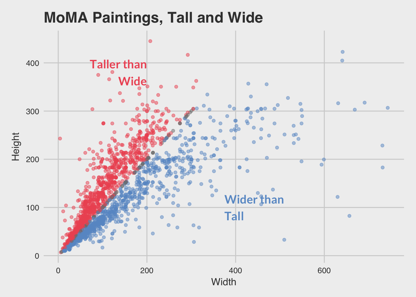

10 Plot something new & different!

Challenge #5:

It can be anything- you can change colors, add annotations, switch the geoms, add new variables to examine- the world is your oyster! The only requirements are:

You make one new plot that is original, and
You write 1-2 sentences to present the plot and why it makes sense. What questions do you think your plot can help you to answer?

It does not have to be pretty right now, but it must make sense as a visualization- you must be able to intelligently and succintly tell us about it in real words.

Lab 02: MoMA Museum Tour

CS631

Alison Hill

1 Goals for Lab 02

2 Slides for today

3 Inspiration + data

4 Packages needed

5 Read in the data

6 Know your data

6.1 How many paintings?

6.2 What is the first painting acquired?

6.3 What is the oldest painting in the MoMA collection?

6.4 How many artists?

6.5 Which artist has the most paintings?

6.6 How many paintings by male vs female artists?

6.7 How many artists of each gender are there?

6.8 When were the most paintings in the collection acquired?

6.9 When were the most paintings in the collection created?

6.10 What about the first painting by a solo female artist?

7 Basics of `ggplot2`

8 Plot your data

8.1 Plot year painted vs year acquired

8.2 Facet by artist gender

9 Plot painting dimensions

10 Plot something new & different!

Lab 02: MoMA Museum Tour

CS631

Alison Hill

1 Goals for Lab 02

2 Slides for today

3 Inspiration + data

4 Packages needed

5 Read in the data

6 Know your data

6.1 How many paintings?

6.2 What is the first painting acquired?

6.3 What is the oldest painting in the MoMA collection?

6.4 How many artists?

6.5 Which artist has the most paintings?

6.6 How many paintings by male vs female artists?

6.7 How many artists of each gender are there?

6.8 When were the most paintings in the collection acquired?

6.9 When were the most paintings in the collection created?

6.10 What about the first painting by a solo female artist?

7 Basics of ggplot2

8 Plot your data

8.1 Plot year painted vs year acquired

8.2 Facet by artist gender

9 Plot painting dimensions

10 Plot something new & different!

7 Basics of `ggplot2`